7 Principles: More Operations

In the previous section we introduced our first few operations to manipulate data frames. Next, we learn a few more: sorting, creating new attributes, summarizing and grouping. Finally we will take a short detour through a discussion on vectors.

7.1 Operations that sort entities

The first operation we will look at today is used to sort entities based on their attribute values. As an example, suppose we wanted to find the arrests with the 10 youngest subjects. If we had an operation that re-orders entities based on the value of their age attribute, we can then use the slice operation we saw before to create a data frame with just the entities of interest

arrest_tab %>%
  arrange(age) %>%
  slice(1:10)

## # A tibble: 10 x 15
##     arrest   age race  sex   arrestDate
##      <dbl> <dbl> <chr> <chr> <chr>     
##  1  1.11e7     0 B     F     01/24/2011
##  2  1.12e7     0 W     M     03/22/2011
##  3 NA          0 <NA>  <NA>  03/28/2011
##  4 NA          0 B     M     03/30/2011
##  5 NA          0 W     F     04/07/2011
##  6  1.12e7     0 W     F     05/20/2011
##  7  1.12e7     0 B     M     06/21/2011
##  8  1.13e7     0 B     M     09/04/2011
##  9  1.13e7     0 B     M     09/28/2011
## 10  1.14e7     0 <NA>  <NA>  12/02/2011
## # … with 10 more variables: arrestTime <time>,
## #   arrestLocation <chr>, incidentOffense <chr>,
## #   incidentLocation <chr>, charge <chr>,
## #   chargeDescription <chr>, district <chr>,
## #   post <dbl>, neighborhood <chr>, `Location
## #   1` <chr>

The arrange operation sorts entities by increasing value of the attributes passed as arguments.

The desc helper function is used to indicate sorting by decreasing value. For example, to find the arrests with the 10 oldest subjects we would use:

arrest_tab %>%
  arrange(desc(age)) %>%
  slice(1:10)

## # A tibble: 10 x 15
##     arrest   age race  sex   arrestDate
##      <dbl> <dbl> <chr> <chr> <chr>     
##  1  1.13e7    87 B     M     08/28/2011
##  2  1.25e7    87 B     M     08/14/2012
##  3  1.12e7    86 B     M     02/22/2011
##  4  1.11e7    85 W     M     01/25/2011
##  5  1.12e7    85 B     M     03/04/2011
##  6  1.14e7    84 B     M     12/27/2011
##  7 NA         84 B     M     01/11/2012
##  8  1.26e7    84 B     M     11/08/2012
##  9  1.12e7    82 B     M     05/17/2011
## 10  1.13e7    80 B     M     09/26/2011
## # … with 10 more variables: arrestTime <time>,
## #   arrestLocation <chr>, incidentOffense <chr>,
## #   incidentLocation <chr>, charge <chr>,
## #   chargeDescription <chr>, district <chr>,
## #   post <dbl>, neighborhood <chr>, `Location
## #   1` <chr>

7.2 Operations that create new attributes

We will often see that for many analyses, be it for interpretation or for statistical modeling, we will create new attributes based on existing attributes in a dataset.

Suppose I want to represent age in months rather than years in our dataset. To do so I would multiply 12 to the existing age attribute. The function mutate creates new attributes based on the result of a given expression:

arrest_tab %>%
  mutate(age_months = 12 * age) %>%
  select(arrest, age, age_months)

## # A tibble: 104,528 x 3
##      arrest   age age_months
##       <dbl> <dbl>      <dbl>
##  1 11126858    23        276
##  2 11127013    37        444
##  3 11126887    46        552
##  4 11126873    50        600
##  5 11126968    33        396
##  6 11127041    41        492
##  7 11126932    29        348
##  8 11126940    20        240
##  9 11127051    24        288
## 10 11127018    53        636
## # … with 104,518 more rows

7.3 Operations that summarize attribute values over entities

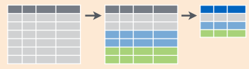
Once we have a set of entities and attributes in a given data frame, we may need to summarize attribute values over the set of entities in the data frame. It collapses the data frame to a single row containing the desired attribute summaries.

Continuing with the example we have seen below, we may want to know what the minmum, maximum and average age in the dataset is:

summarize(arrest_tab, min_age=min(age), mean_age=mean(age), max_age=max(age))

## # A tibble: 1 x 3
##   min_age mean_age max_age
##     <dbl>    <dbl>   <dbl>
## 1       0     33.2      87

The summarize functions takes a data frame and calls a summary function over attributes of the data frame. Common summary functions to use include:

Operation(s)	Result
`mean`, `median`	average and median attribute value, respectively
`sd`	standard deviation of attribute values
`min`, `max`	minimum and maximum attribute values, respectively
`n`, `n_distinct`	number of attribute values and number of distinct attribute values
`any`, `all`	for logical attributes (TRUE/FALSE): is `any` attribute value TRUE, or are `all` attribute values TRUE

Let’s see the number of distinct districts in our dataset:

summarize(arrest_tab, n_distinct(district))

## # A tibble: 1 x 1
##   `n_distinct(district)`
##                    <int>
## 1                     10

We may also refer to these summarization operation as aggregation since we are computing aggregates of attribute values.

7.4 Operations that group entities

Summarization (therefore aggregation) goes hand in hand with data grouping, where summaries are computed conditioned on other attributes. The notion of conditioning is fundamental to data analysis and we will see it very frequently through the course. It is the basis of statistical analysis and Machine Learning models and it is essential in understanding the design of effective visualizations.

The goal is to group entities with the same value of one or more attributes. The group_by function in essence annotates the rows of a data frame as belonging to a specific group based on the value of some chosen attributes. This call returns a data frame that is grouped by the value of the district attribute.

group_by(arrest_tab, district)

## # A tibble: 104,528 x 15
## # Groups:   district [10]
##    arrest   age race  sex   arrestDate arrestTime
##     <dbl> <dbl> <chr> <chr> <chr>      <time>    
##  1 1.11e7    23 B     M     01/01/2011 00'00"    
##  2 1.11e7    37 B     M     01/01/2011 01'00"    
##  3 1.11e7    46 B     M     01/01/2011 01'00"    
##  4 1.11e7    50 B     M     01/01/2011 04'00"    
##  5 1.11e7    33 B     M     01/01/2011 05'00"    
##  6 1.11e7    41 B     M     01/01/2011 05'00"    
##  7 1.11e7    29 B     M     01/01/2011 05'00"    
##  8 1.11e7    20 W     M     01/01/2011 05'00"    
##  9 1.11e7    24 B     M     01/01/2011 07'00"    
## 10 1.11e7    53 B     M     01/01/2011 15'00"    
## # … with 104,518 more rows, and 9 more
## #   variables: arrestLocation <chr>,
## #   incidentOffense <chr>,
## #   incidentLocation <chr>, charge <chr>,
## #   chargeDescription <chr>, district <chr>,
## #   post <dbl>, neighborhood <chr>, `Location
## #   1` <chr>

Subsequent operations are then performed for each group independently. For example, when summarize is applied to a grouped data frame, summaries are computed for each group of entities, rather than the whole set of entities.

For instance, let’s calculate minimum, maximum and average age for each district in our dataset:

arrest_tab %>%
  group_by(district) %>%
  summarize(min_age=min(age), max_age=max(age), mean_age=mean(age))

## # A tibble: 10 x 4
##    district     min_age max_age mean_age
##    <chr>          <dbl>   <dbl>    <dbl>
##  1 CENTRAL            0      86     33.0
##  2 EASTERN            0      85     34.1
##  3 NORTHEASTERN       0      78     30.4
##  4 NORTHERN          14      80     33.1
##  5 NORTHWESTERN       0      78     34.6
##  6 SOUTHEASTERN       0      87     32.5
##  7 SOUTHERN           0      84     32.3
##  8 SOUTHWESTERN       0      80     32.4
##  9 WESTERN            0      73     34.4
## 10 <NA>               0      87     33.4

Note that after this operation we have effectively changed the entities represented in the result. The entities in our original dataset are arrests while the entities for the result of the last example are the districts. This is a general property of group_by and summarize: it defines a data set where entities are defined by distinct values of the attributes we use for grouping.

Let’s look at another example combining some of the operations we have seen so far. Let’s compute the average age for subjects 21 years or older grouped by district and sex:

arrest_tab %>%
  filter(age >= 21) %>%
  group_by(district, sex) %>%
  summarize(mean_age=mean(age))

## # A tibble: 20 x 3
## # Groups:   district [10]
##    district     sex   mean_age
##    <chr>        <chr>    <dbl>
##  1 CENTRAL      F         35.7
##  2 CENTRAL      M         35.3
##  3 EASTERN      F         36.9
##  4 EASTERN      M         37.1
##  5 NORTHEASTERN F         33.5
##  6 NORTHEASTERN M         32.8
##  7 NORTHERN     F         35.9
##  8 NORTHERN     M         35.6
##  9 NORTHWESTERN F         37.5
## 10 NORTHWESTERN M         37.2
## 11 SOUTHEASTERN F         33.3
## 12 SOUTHEASTERN M         34.7
## 13 SOUTHERN     F         33.7
## 14 SOUTHERN     M         34.5
## 15 SOUTHWESTERN F         35.4
## 16 SOUTHWESTERN M         35.0
## 17 WESTERN      F         37.1
## 18 WESTERN      M         37.3
## 19 <NA>         F         34.7
## 20 <NA>         M         35.5

Exercise: Write a data operation pipeline that

filters records to the southern district and ages between 18 and 25
computes mean arrest age for each sex

7.5 Vectors

We briefly saw previously operators to create vectors in R. For instance, we can use seq to create a vector that consists of a sequence of integers:

multiples_of_three <- seq(3, 30, by=3)
multiples_of_three

##  [1]  3  6  9 12 15 18 21 24 27 30

Let’s how this is represented in R (the str is very handy to do this type of digging around):

str(multiples_of_three)

##  num [1:10] 3 6 9 12 15 18 21 24 27 30

So, this is a numeric vector of length 10. Like many other languages we use square brackets [] to index vectors:

multiples_of_three[1]

## [1] 3

We can use ranges as before

multiples_of_three[1:4]

## [1]  3  6  9 12

We can use vectors of non-negative integers for indexing:

multiples_of_three[c(1,3,5)]

## [1]  3  9 15

Or even logical vectors:

multiples_of_three[c(TRUE, FALSE, TRUE, FALSE, TRUE, FALSE, TRUE, FALSE, TRUE, FALSE)]

## [1]  3  9 15 21 27

In R, most operations are designed to work with vectors directly (we call that vectorized). For example, if I want to add two vectors together I would write: (look no for loop!):

multiples_of_three + multiples_of_three

##  [1]  6 12 18 24 30 36 42 48 54 60

This also works for other arithmetic and logical operations (e.g., -, *, /, &, |). Give them a try!

In data analysis the vector is probably the most fundamental data type (other than basic numbers, strings, etc.). Why? Consider getting data about one attribute, say height, for a group of people. What do you get? An array of numbers, all in the same unit (say feet, inches or centimeters). How about their name? Then you get an array of strings. Abstractly, we think of vectors as arrays of values, all of the same class or datatype.

7.6 Attributes as vectors

In fact, in the data frames we have been working on, each column, corresponding to an attribute, is a vector. We use the pull function to extract a vector from a data frame. We can then operate index them, or operate on them as vectors

age_vec <- arrest_tab %>% pull(age)
age_vec[1:10]

##  [1] 23 37 46 50 33 41 29 20 24 53

12 * age_vec[1:10]

##  [1] 276 444 552 600 396 492 348 240 288 636

We previously saw how the $ operator serves the same function.

age_vec <- arrest_tab$age
age_vec[1:10]

##  [1] 23 37 46 50 33 41 29 20 24 53

The pull function however, can be used as part of a pipeline (using operator %>%):

arrest_tab %>%
  pull(age) %>%
  mean()

## [1] 33.19639

7.7 Functions

Once we have established useful pipelines for a dataset we will want to abstract them into reusable functions that we can apply in other analyses. To do that we would write our own functions that encapsulate the pipelines we have created. As an example, take a function that executes the age by district/sex summarization we created before:

summarize_district <- function(df) {
  df %>%
    filter(age >= 21) %>%
    group_by(district, sex) %>%
    summarize(mean_age=mean(age))
}

You can include multiple expressions in the function definition (inside brackets {}). Notice there is no return statement in this function. When a function is called, it returns the value of the last expression in the function definition. In this example, it would be the data frame we get from applying the pipeline of operations.

You can find more information about vectors, functions and other programming matters we might run into in class in Chapters 17-21 of R for Data Science

Exercise Abstract the pipeline you wrote in the previous unit into a function that works for arbitrary districts. The function should take arguments df and district.