15 DB Parting Shots
15.1 Database Query Optimization
Earlier we made the distinction that SQL is a declarative language rather than a procedural language. A reason why data base systems rely on a declarative language is that it allows the system to decide how to evaluate a query most efficiently. Let’s think about this briefly.
Consider a database where we have two tables Batting and Master and we want to evaluate this query: that what is the maximum batting “average” for a player from the state of California?
select max(1.0 * b.H / b.AB) as best_ba
from Batting as b join Master as m on b.playerId = m.playerId
where b.AB >= 100 and m.birthState = "CA"
Now, let’s do the same computation using dplyr operations:
Here is one version that joins the two tables before filtering the rows that are included in the result.
Batting %>%
  inner_join(Master, by="playerID") %>%
  filter(AB >= 100, birthState == "CA") %>%
  mutate(AB=1.0 * H / AB) %>%
  summarize(max(AB))
## max(AB)
## 1 0.4057018Here is a second version that filters the rows of the tables before joining the two tables.
Batting %>%
  filter(AB >= 100) %>%
  inner_join(
    Master %>% filter(birthState == "CA")
  ) %>%
  mutate(AB = 1.0 * H / AB) %>%
  summarize(max(AB))
## Joining, by = "playerID"## max(AB)
## 1 0.4057018They both give the same result of course, but which one should be more efficient?
Let’s think about this with a very simple cost model of how efficient each of these two procedural versions will be. The costliest operation here is the join between two tables. Let’s take the simplest algorithm we can to compute the join T1 %>% inner_join(T2, by="A") where T1 and T2 are the tables to join and A the attribute we are using to join the two tables.
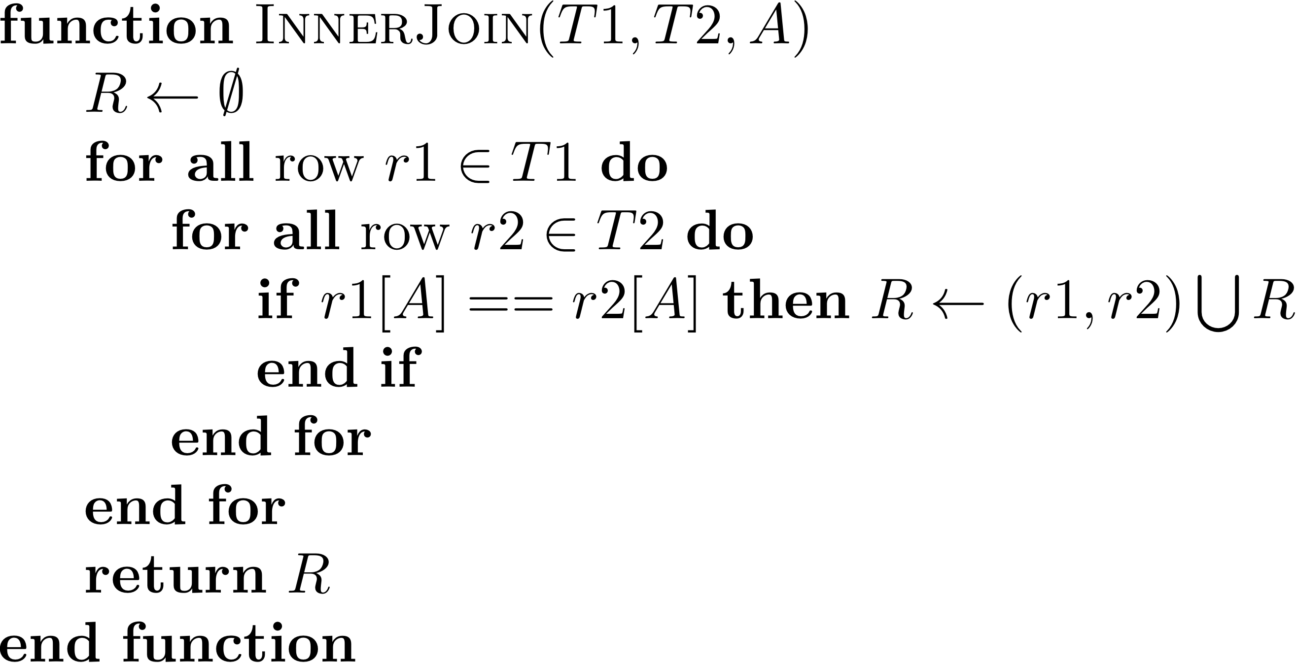
What is the cost of this algorithm? \(|T1| \times |T2|\). For the rest of the operations, let’s assume we perform this with a single pass through the table. For example, we assume that filter(T) has cost \(|T|\).
Under these assumptions, let’s write out the cost of each of the two pipelines we wrote above.
Batting %>%
  inner_join(Master, by="playerID") %>% # cost: |Batting| x |Master|
  filter(AB >= 100, birthState == "CA") %>% # cost: |R1|
  mutate(AB=1.0 * H / AB) %>% # cost: |R|
  summarize(max(AB)) # cost: |R|
So, cost here is \(|\mathrm{Batting}|\times|\mathrm{Master}| + |R1| + 2|R|\) where \(R1\) is the table resulting from the inner join between Batting and Master and \(R\) is \(R\) filtered to rows with AB >=100 & birthState == "CA". We can compute this:
batting_size <- nrow(Batting)
master_size <- nrow(Master)

r1 <- Batting %>% inner_join(Master, by="playerID")
r1_size <- nrow(r1)

r <- filter(r1, AB>=100, birthState == "CA")
r_size <- nrow(r)

total_cost_v1 <- batting_size * master_size + r1_size + 2*r_size
total_cost_v1
## [1] 2076791824Now, let’s look at the second version.
Batting %>%
  filter(AB >= 100) %>% # cost: |Batting|
  inner_join(
    Master %>% filter(birthState == "CA") # cost: |Master|
  ) %>% # cost: |B1| x |M1|
  mutate(AB = 1.0 * H / AB) %>% # cost |R|
  summarize(max(AB)) # cost |R|
So, cost here is \(|\mathrm{Batting}| \times |\mathrm{Master}| + |B1|\times|M1|+2|R|\) where \(B1\) is the Batting table filtered to include only rows with AB >= 100, and \(M2\) is the Master table filtered to include
birthState == "CA". Let’s compute this:
b1 <- filter(Batting, AB>=100)
b1_size <- nrow(b1)

m1 <- filter(Master, birthState == "CA")
m1_size <- nrow(m1)

total_cost_v2 <- batting_size + master_size + b1_size * m1_size + 2*r_size
total_cost_v2
## [1] 89525504In this case, the procedural version that joins tables before filtering is 23 times costlier. When using SQL in a database system we only write the one query describing our desired result, with the procedural versions with dplyr we need to think which of the two versions is more efficient.
Database systems use query optimization to decide how to evaluate queries efficiently. The goal of query optimization is to decide the most efficient query plan to use to evaluate a query out of the many possible candidate plans it could use. It needs to solve two problems: search the space of possible plans, approximate the cost of evaluating a specific plan. Let’s ignore the first, and discuss briefly the second.
We should think of the two procedural versions above as two candidate plans that the DB system could use to evaluate the query. Query optimzation approximates what it would cost to evaluate each of the two plans and decides to use the most efficient plan.
So, how does it approximate cost? A few ingredients are used:
Access cost: how much will it cost to access rows that satisfy a given predicate (
whereclause)? Consider theMastertable. In our query we only need to find rows for players born in California. Suppose we have an index based on attributebirthState, e.g. a hash table that allows us to find rows for players from a specific state very efficiently. In that case, accessing these rows using the index is much more efficient than scanning the entire table. This is why creating indexes for tables becomes important.Operation cost: how much will it cost to perform a join? There is a difference between comparing every pair of rows in order to compute a join, versus using indexes to find a small number of rows that satisfy the join condition efficiently? For example, if the
Battingtable has an index onplayerIdit will be cheaper to join with a filteredMastertable, i.e., only considering rows for players born in California.Result size estimation: how many rows will we get after we perform a join? We can use information on key constraints to estimate this type of result. Additionally, these estimates also depend on the number of rows that satisfy certain predicates (e.g., number of players born in California) so systems often use histograms to make these estimates.
As database system users we may create indices or key constraints that guide the query optimizer to choose more efficient queries.
15.2 JSON Data Model
The Entity-Relational data model we have described so far is mostly defined for structured data: where a specific and consistent schema is assumed.
Data models like XML and JSON are instead intended for semi-structured data.
15.2.0.1 XML: eXtensible Markup Language
Data models like XML rely on flexible, self-describing schemas:
<?xml version="1.0" encoding="UTF-8"?>
<!-- Edited by XMLSpy -->
<CATALOG>
  <CD>
    <TITLE>Empire Burlesque</TITLE>
    <ARTIST>Bob Dylan</ARTIST>
    <COUNTRY>USA</COUNTRY>
    <COMPANY>Columbia</COMPANY>
    <PRICE>10.90</PRICE>
    <YEAR>1985</YEAR>
  </CD>
  <CD>
    <TITLE>Hide your heart</TITLE>
    <ARTIST>Bonnie Tyler</ARTIST>
    <COUNTRY>UK</COUNTRY>
    <COMPANY>CBS Records</COMPANY>
    <PRICE>9.90</PRICE>
    <YEAR>1988</YEAR>
  </CD>
  ...
15.2.0.2 JSON: Javascript Object Notation
Very similar to XML and seems to be replacing it for many purposes
{
  "firstName": "John",
  "lastName": "Smith",
  "isAlive": true,
  "age": 25,
  "height_cm": 167.6,
  "address": {
    "streetAddress": "21 2nd Street",
    "city": "New York",
    "state": "NY",
    "postalCode": "10021-3100"
  },
  "phoneNumbers": [
    {
      "type": "home",
      "number": "212 555-1234"
    },
    {
      "type": "office",
      "number": "646 555-4567"
    }
  ],
  "children": [],
  "spouse": null
}
This is the format most contemporary data REST APIs use to transfer data. For instance, here is part of a JSON record from a Twitter stream:
{
  "created_at":"Sun May 05 14:01:34+00002013",
  "id":331046012875583488,
  "id_str":"331046012875583488",
  "text":"\u0425\u043e\u0447\u0443, \u0447\u0442\u043e\u0431 \u0442\u044b \u0441\u0434\u0435\u043b\u0430\u043b \u0432\u0441\u0451 \u043d\u0435\u043e\u0431\u0445\u043e\u0434\u0438\u043c\u043e\u0435.\n \\,,\\ *_* \/,,\/",
  "source":"\u003ca href=\"http:\/\/twitterfeed.com\"rel=\"nofollow\"\u003etwitterfeed\u003c\/a\u003e",
  "in_reply_to_user_id_str":null,
  "user":{
    "id":548422428,
    "id_str":"548422428",
    "name":"\u0410\u0439\u0433\u0435\u0440\u0438\u043c \u041f\u043e\u0433\u043e\u0434\u0438\u043d\u0430",
    "screen_name":"paddybyrny",
    "location":"\u0420\u043e\u0441\u0441\u0438\u044f;\u0412\u043b\u0430\u0434\u0438\u0432\u043e\u0441\u0442\u043e\u043a",
    "followers_count":4188,
    "friends_count":4281,
    "lang":"en",
    "profile_background_image_url":"http:\/\/a0.twimg.com\/images\/themes\/theme1\/bg.png",
  },
  "geo":null,
  "coordinates":null,
  "entities":{
    "hashtags":[],"symbols":[],"urls":[],"user_mentions":[]
  },"favorited":false,"retweeted":false,"filter_level":"medium","lang":"ru"}