6 Principles: Basic Operations
Now that we have a data frame describing our data, let’s learn a few fundamental operations we perform on data frames on almost any analysis. We divide these first set of operations into two groups: operations on attributes and operations on entitites. These operations are defined in the dplyr package, part of the tidyverse, and are described in more detail in the “R for Data Science” textbook available in the course logistics page: http://r4ds.had.co.nz/transform.html.
6.1 Operations that subset attributes
6.1.1 select
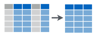
In our data set we have a large number of attributes describing each arrest. Now, suppose we only want to study patterns in these arrests based on a smaller number of attributes for purposes of efficiency, since we would operate over less data, or interpretability. In that case we would like to create a data frame that contains only those attributes of interest. We use the select function for this.
Let’s create a data frame containing only the age, sex and district attributes
## # A tibble: 104,528 x 3
##      age sex   district
##    <dbl> <fct> <chr>
##  1    23 M     <NA>
##  2    37 M     SOUTHERN
##  3    46 M     NORTHEASTERN
##  4    50 M     WESTERN
##  5    33 M     NORTHERN
##  6    41 M     SOUTHERN
##  7    29 M     WESTERN
##  8    20 M     NORTHEASTERN
##  9    24 M     <NA>
## 10    53 M     NORTHWESTERN
## # … with 104,518 more rows
The first argument to the select function is the data frame we want to operate on, the remaining arguments describe the attributes we want to include in the resulting data frame.
Note a few other things:
The first argument to
selectis a data frame, and the value returned byselectis also a data frameAs always you can learn more about the function using
?select
Attribute descriptor arguments can be fairly sophisticated. For example, we can use positive integers to indicate attribute (column) indices:
## # A tibble: 104,528 x 3
##      arrest race  sex
##       <dbl> <chr> <fct>
##  1 11126858 B     M
##  2 11127013 B     M
##  3 11126887 B     M
##  4 11126873 B     M
##  5 11126968 B     M
##  6 11127041 B     M
##  7 11126932 B     M
##  8 11126940 W     M
##  9 11127051 B     M
## 10 11127018 B     M
## # … with 104,518 more rows
R includes a useful operator to describe ranges. E.g., 1:5 would be attributes 1 through 5:
## # A tibble: 104,528 x 5
##      arrest   age race  sex   arrestDate
##       <dbl> <dbl> <chr> <fct> <chr>
##  1 11126858    23 B     M     01/01/2011
##  2 11127013    37 B     M     01/01/2011
##  3 11126887    46 B     M     01/01/2011
##  4 11126873    50 B     M     01/01/2011
##  5 11126968    33 B     M     01/01/2011
##  6 11127041    41 B     M     01/01/2011
##  7 11126932    29 B     M     01/01/2011
##  8 11126940    20 W     M     01/01/2011
##  9 11127051    24 B     M     01/01/2011
## 10 11127018    53 B     M     01/01/2011
## # … with 104,518 more rows
We can also use other helper functions to create attribute descriptors. For example, to choose all attributes that begin with the letter a we can the starts_with function which uses partial string matching:
## # A tibble: 104,528 x 5
##    arrest   age arrestDate arrestTime
##     <dbl> <dbl> <chr>      <time>
##  1 1.11e7    23 01/01/2011 00'00"
##  2 1.11e7    37 01/01/2011 01'00"
##  3 1.11e7    46 01/01/2011 01'00"
##  4 1.11e7    50 01/01/2011 04'00"
##  5 1.11e7    33 01/01/2011 05'00"
##  6 1.11e7    41 01/01/2011 05'00"
##  7 1.11e7    29 01/01/2011 05'00"
##  8 1.11e7    20 01/01/2011 05'00"
##  9 1.11e7    24 01/01/2011 07'00"
## 10 1.11e7    53 01/01/2011 15'00"
## # … with 104,518 more rows, and 1 more variable:
## #   arrestLocation <chr>
We can also use the attribute descriptor arguments to drop attributes. For instance using descriptor -age returns the arrest data frame with all but the age attribute included:
## # A tibble: 104,528 x 14
##    arrest race  sex   arrestDate arrestTime
##     <dbl> <chr> <fct> <chr>      <time>
##  1 1.11e7 B     M     01/01/2011 00'00"
##  2 1.11e7 B     M     01/01/2011 01'00"
##  3 1.11e7 B     M     01/01/2011 01'00"
##  4 1.11e7 B     M     01/01/2011 04'00"
##  5 1.11e7 B     M     01/01/2011 05'00"
##  6 1.11e7 B     M     01/01/2011 05'00"
##  7 1.11e7 B     M     01/01/2011 05'00"
##  8 1.11e7 W     M     01/01/2011 05'00"
##  9 1.11e7 B     M     01/01/2011 07'00"
## 10 1.11e7 B     M     01/01/2011 15'00"
## # … with 104,518 more rows, and 9 more
## #   variables: arrestLocation <chr>,
## #   incidentOffense <chr>,
## #   incidentLocation <chr>, charge <chr>,
## #   chargeDescription <chr>, district <chr>,
## #   post <dbl>, neighborhood <chr>, `Location
## #   1` <chr>
6.1.2 rename
To improve interpretability during an analysis we may want to rename attributes. We use the rename function for this:
## # A tibble: 104,528 x 15
##    arrest   age race  sex   arrest_date
##     <dbl> <dbl> <chr> <fct> <chr>
##  1 1.11e7    23 B     M     01/01/2011
##  2 1.11e7    37 B     M     01/01/2011
##  3 1.11e7    46 B     M     01/01/2011
##  4 1.11e7    50 B     M     01/01/2011
##  5 1.11e7    33 B     M     01/01/2011
##  6 1.11e7    41 B     M     01/01/2011
##  7 1.11e7    29 B     M     01/01/2011
##  8 1.11e7    20 W     M     01/01/2011
##  9 1.11e7    24 B     M     01/01/2011
## 10 1.11e7    53 B     M     01/01/2011
## # … with 104,518 more rows, and 10 more
## #   variables: arrestTime <time>,
## #   arrestLocation <chr>, incidentOffense <chr>,
## #   incidentLocation <chr>, charge <chr>,
## #   chargeDescription <chr>, district <chr>,
## #   post <dbl>, neighborhood <chr>, `Location
## #   1` <chr>
Like select, the first argument to the function is the data frame we are operating on. The remaining arguemnts specify attributes to rename and the name they will have in the resulting data frame. Note that arguments in this case are named (have the form lhs=rhs). We can have selection and renaming by using named arguments in select:
## # A tibble: 104,528 x 3
##      age sex   arrest_date
##    <dbl> <fct> <chr>
##  1    23 M     01/01/2011
##  2    37 M     01/01/2011
##  3    46 M     01/01/2011
##  4    50 M     01/01/2011
##  5    33 M     01/01/2011
##  6    41 M     01/01/2011
##  7    29 M     01/01/2011
##  8    20 M     01/01/2011
##  9    24 M     01/01/2011
## 10    53 M     01/01/2011
## # … with 104,518 more rows
Also like select, the result of calling rename is a data frame. In fact, this will be the case for almost all operations in the tidyverse they operate on data frames (specified as the first
ment in the function call) and return data frames.
6.2 Operations that subset entities
Next, we look at operations that select entities from a data frame. We will see a few operations to do this: selecting specific entities (rows) by position, selecting them based on attribute properties, and random sampling.

6.2.1 slice
We can choose specific entities by their row position. For instance, to choose entities in rows 1,3 and 10, we would use the following:
## # A tibble: 3 x 15
##   arrest   age race  sex   arrestDate arrestTime
##    <dbl> <dbl> <chr> <fct> <chr>      <time>
## 1 1.11e7    23 B     M     01/01/2011 00'00"
## 2 1.11e7    46 B     M     01/01/2011 01'00"
## 3 1.11e7    53 B     M     01/01/2011 15'00"
## # … with 9 more variables: arrestLocation <chr>,
## #   incidentOffense <chr>,
## #   incidentLocation <chr>, charge <chr>,
## #   chargeDescription <chr>, district <chr>,
## #   post <dbl>, neighborhood <chr>, `Location
## #   1` <chr>
As before, the first argument is the data frame to operate on. The second argument is a vector of indices. We used the c function (for concatenate) to create a vector of indices.
We can also use the range operator here:
## # A tibble: 5 x 15
##   arrest   age race  sex   arrestDate arrestTime
##    <dbl> <dbl> <chr> <fct> <chr>      <time>
## 1 1.11e7    23 B     M     01/01/2011 00'00"
## 2 1.11e7    37 B     M     01/01/2011 01'00"
## 3 1.11e7    46 B     M     01/01/2011 01'00"
## 4 1.11e7    50 B     M     01/01/2011 04'00"
## 5 1.11e7    33 B     M     01/01/2011 05'00"
## # … with 9 more variables: arrestLocation <chr>,
## #   incidentOffense <chr>,
## #   incidentLocation <chr>, charge <chr>,
## #   chargeDescription <chr>, district <chr>,
## #   post <dbl>, neighborhood <chr>, `Location
## #   1` <chr>
To create general sequences of indices we would use the seq function. For example, to select entities in even positions we would use the following:
## # A tibble: 52,264 x 15
##    arrest   age race  sex   arrestDate arrestTime
##     <dbl> <dbl> <chr> <fct> <chr>      <time>
##  1 1.11e7    37 B     M     01/01/2011 01'00"
##  2 1.11e7    50 B     M     01/01/2011 04'00"
##  3 1.11e7    41 B     M     01/01/2011 05'00"
##  4 1.11e7    20 W     M     01/01/2011 05'00"
##  5 1.11e7    53 B     M     01/01/2011 15'00"
##  6 1.11e7    25 B     M     01/01/2011 20'00"
##  7 1.11e7    50 B     M     01/01/2011 40'00"
##  8 1.11e7    40 B     M     01/01/2011 40'00"
##  9 1.11e7    30 B     M     01/01/2011 40'00"
## 10 1.11e7    53 B     M     01/01/2011 40'00"
## # … with 52,254 more rows, and 9 more variables:
## #   arrestLocation <chr>, incidentOffense <chr>,
## #   incidentLocation <chr>, charge <chr>,
## #   chargeDescription <chr>, district <chr>,
## #   post <dbl>, neighborhood <chr>, `Location
## #   1` <chr>
6.2.2 filter
We can also select entities based on attribute properties. For example, to select arrests where age is less than 18 years old, we would use the following:
## # A tibble: 463 x 15
##    arrest   age race  sex   arrestDate arrestTime
##     <dbl> <dbl> <chr> <fct> <chr>      <time>
##  1 1.11e7    17 B     M     01/03/2011 15:00
##  2 1.11e7    17 B     M     01/07/2011 18:40
##  3 1.11e7    17 A     M     01/10/2011 22:00
##  4 1.11e7    17 B     M     01/13/2011 01:00
##  5 1.11e7    17 B     F     01/13/2011 13:40
##  6 1.11e7    17 B     M     01/13/2011 18:40
##  7 1.11e7    14 B     M     01/17/2011 21:57
##  8 1.11e7    17 B     M     01/18/2011 15:00
##  9 1.11e7    17 B     M     01/18/2011 15:26
## 10 1.11e7    16 B     M     01/18/2011 16:00
## # … with 453 more rows, and 9 more variables:
## #   arrestLocation <chr>, incidentOffense <chr>,
## #   incidentLocation <chr>, charge <chr>,
## #   chargeDescription <chr>, district <chr>,
## #   post <dbl>, neighborhood <chr>, `Location
## #   1` <chr>
You know by now what the first argument is…
The second argument is an expression that evaluates to a logical value (TRUE or FALSE), if the expression evaluates to TRUE for a given entity (row) then that entity (row) is part of the resulting data frame. Operators used frequently include:
==, !=: tests equality and inequality respectively (categorical, numerical, datetimes, etc.)
<, >, <=, >=: tests order relationships for ordered data types (not categorical)
!, &, |: not, and, or, logical operators
To select arrests with ages between 18 and 25 we can use
## # A tibble: 35,770 x 15
##    arrest   age race  sex   arrestDate arrestTime
##     <dbl> <dbl> <chr> <fct> <chr>      <time>
##  1 1.11e7    23 B     M     01/01/2011 00:00
##  2 1.11e7    20 W     M     01/01/2011 00:05
##  3 1.11e7    24 B     M     01/01/2011 00:07
##  4 1.11e7    25 B     M     01/01/2011 00:20
##  5 1.11e7    24 B     M     01/01/2011 00:40
##  6 1.11e7    20 B     M     01/01/2011 01:22
##  7 1.11e7    23 B     M     01/01/2011 01:30
##  8 1.11e7    22 A     M     01/01/2011 01:40
##  9 1.11e7    20 W     M     01/01/2011 02:00
## 10 1.11e7    20 B     M     01/01/2011 02:20
## # … with 35,760 more rows, and 9 more variables:
## #   arrestLocation <chr>, incidentOffense <chr>,
## #   incidentLocation <chr>, charge <chr>,
## #   chargeDescription <chr>, district <chr>,
## #   post <dbl>, neighborhood <chr>, `Location
## #   1` <chr>
The filter function can take multiple logical expressions. In this case they are combined with &. So the above is equivalent to
## # A tibble: 35,770 x 15
##    arrest   age race  sex   arrestDate arrestTime
##     <dbl> <dbl> <chr> <fct> <chr>      <time>
##  1 1.11e7    23 B     M     01/01/2011 00:00
##  2 1.11e7    20 W     M     01/01/2011 00:05
##  3 1.11e7    24 B     M     01/01/2011 00:07
##  4 1.11e7    25 B     M     01/01/2011 00:20
##  5 1.11e7    24 B     M     01/01/2011 00:40
##  6 1.11e7    20 B     M     01/01/2011 01:22
##  7 1.11e7    23 B     M     01/01/2011 01:30
##  8 1.11e7    22 A     M     01/01/2011 01:40
##  9 1.11e7    20 W     M     01/01/2011 02:00
## 10 1.11e7    20 B     M     01/01/2011 02:20
## # … with 35,760 more rows, and 9 more variables:
## #   arrestLocation <chr>, incidentOffense <chr>,
## #   incidentLocation <chr>, charge <chr>,
## #   chargeDescription <chr>, district <chr>,
## #   post <dbl>, neighborhood <chr>, `Location
## #   1` <chr>
6.2.3 sample_n and sample_frac
Frequently we will want to choose entities from a data frame at random. The sample_n function selects a specific number of entities at random:
## # A tibble: 10 x 15
##     arrest   age race  sex   arrestDate
##      <dbl> <dbl> <chr> <fct> <chr>
##  1  1.12e7    41 B     M     06/08/2011
##  2  1.26e7    28 B     M     12/12/2012
##  3  1.25e7    21 B     M     07/31/2012
##  4  1.14e7    26 B     M     11/13/2011
##  5  1.13e7    55 B     M     08/31/2011
##  6  1.14e7    25 B     M     11/12/2011
##  7 NA         22 B     F     03/09/2011
##  8  1.26e7    24 B     M     10/31/2012
##  9 NA         37 B     M     05/27/2011
## 10  1.26e7    40 B     M     11/13/2012
## # … with 10 more variables: arrestTime <time>,
## #   arrestLocation <chr>, incidentOffense <chr>,
## #   incidentLocation <chr>, charge <chr>,
## #   chargeDescription <chr>, district <chr>,
## #   post <dbl>, neighborhood <chr>, `Location
## #   1` <chr>
The sample_frac function selects a fraction of entitites at random:
## # A tibble: 10,453 x 15
##    arrest   age race  sex   arrestDate arrestTime
##     <dbl> <dbl> <chr> <fct> <chr>      <time>
##  1 1.13e7    53 B     M     07/27/2011 09:12
##  2 1.12e7    25 B     M     04/06/2011 19:45
##  3 1.26e7    20 B     M     10/08/2012 17:45
##  4 1.14e7    19 B     M     11/30/2011 19:30
##  5 1.25e7    25 B     M     08/11/2012 18:00
##  6 1.12e7    25 B     M     05/24/2011 18:45
##  7 1.12e7    20 B     M     02/26/2011 12:16
##  8 1.24e7    44 B     M     01/10/2012 13:30
##  9 1.25e7    20 B     M     06/19/2012 23:53
## 10 1.12e7    41 B     M     03/19/2011 15:00
## # … with 10,443 more rows, and 9 more variables:
## #   arrestLocation <chr>, incidentOffense <chr>,
## #   incidentLocation <chr>, charge <chr>,
## #   chargeDescription <chr>, district <chr>,
## #   post <dbl>, neighborhood <chr>, `Location
## #   1` <chr>
6.3 Pipelines of operations
All of the functions implementing our first set of operations have the same argument/value structure. They take a data frame as a first argument and return a data frame. We refer to this as the data–>transform–>data pattern. This is the core a lot of what we will do in class as part of data analyses. Specifically, we will combine operations into pipelines that manipulate data frames.
The dplyr package introduces syntactic sugar to make this pattern explicit. For instance, we can rewrite the sample_frac example using the “pipe” operator %>%:
## # A tibble: 10,453 x 15
##     arrest   age race  sex   arrestDate
##      <dbl> <dbl> <chr> <fct> <chr>
##  1  1.12e7    22 B     M     02/18/2011
##  2  1.26e7    58 B     M     11/30/2012
##  3 NA         28 W     F     08/22/2012
##  4  1.24e7    38 B     F     01/08/2012
##  5  1.24e7    22 B     M     03/22/2012
##  6  1.25e7    43 B     F     04/06/2012
##  7  1.12e7    21 B     F     05/11/2011
##  8  1.25e7    25 B     M     07/20/2012
##  9  1.13e7    18 B     M     10/07/2011
## 10  1.25e7    19 B     M     09/01/2012
## # … with 10,443 more rows, and 10 more
## #   variables: arrestTime <time>,
## #   arrestLocation <chr>, incidentOffense <chr>,
## #   incidentLocation <chr>, charge <chr>,
## #   chargeDescription <chr>, district <chr>,
## #   post <dbl>, neighborhood <chr>, `Location
## #   1` <chr>
The %>% binary operator takes the value to its left and inserts it as the first argument of the function call to its right. So the expression LHS %>% f(another_argument) is equivalent to the expression f(LHS, another_argument).
Using the %>% operator and the data–>transform–>data pattern of the functions we’ve seen so far, we can create pipelines. For example, let’s create a pipeline that:
- filters our dataset to arrests between the ages of 18 and 25
- selects attributes
sex,districtandarrestDate(renamed asarrest_date) - samples 50% of those arrests at random
We will assign the result to variable analysis_tab
analysis_tab <- arrest_tab %>%
  filter(age >= 18, age <= 25) %>%
  select(sex, district, arrest_date=arrestDate) %>%
  sample_frac(.5)
analysis_tab
## # A tibble: 17,885 x 3
## sex district arrest_date
## <fct> <chr> <chr>
## 1 F EASTERN 11/02/2011
## 2 F SOUTHWESTERN 11/02/2011
## 3 M EASTERN 11/21/2012
## 4 M <NA> 10/26/2011
## 5 M SOUTHEASTERN 05/24/2012
## 6 M EASTERN 03/20/2012
## 7 M WESTERN 09/13/2011
## 8 M EASTERN 06/24/2011
## 9 F <NA> 10/16/2012
## 10 M <NA> 02/21/2011
## # … with 17,875 more rowsExercise: Create a pipeline that:
- filters dataset to arrests from the “SOUTHERN” district occurring before “12:00” (
arrestTime) - selects attributes,
sex,age - samples 10 entities at random