16 Ingesting data
Now that we have a better understanding of data analysis languages with tidyverse and SQL, we turn to the first significant challenge in data analysis, getting data into R in a shape that we can use to start our analysis. We will look at two types of data ingestion: structured ingestion, where we read data that is already structured, like a comma separated value (CSV) file, and scraping where we obtain data from text, usually in websites.
There is an excellent discussion on data import here: http://r4ds.had.co.nz/data-import.html
16.1 Structured ingestion
16.1.1 CSV files (and similar)
We saw in a previous chapter how we can use the read_csv file to read data from a CSV file into a data frame. Comma separated value (CSV) files are structured in a somewhat regular way, so reading into a data frame is straightforward. Each line in the CSV file corresponds to an observation (a row in a data frame). Each line contains values separated by a comma (,), corresponding to the variables of each observation.
This ideal principle of how a CSV file is constructed is frequently violated by data contained in CSV files. To get a sense of how to deal with these cases look at the documentation of the read_csv function. For instance:
the first line of the file may or may not contain the names of variables for the data frame (
col_namesargument).strings are quoted using
'instead of"(quoteargument)missing data is encoded with a non-standard code, e.g.,
-(naargument)values are separated by a character other than
,(read_delimfunction)file may contain header information before the actual data so we have to skip some lines when loading the data (
skipargument)
You should read the documentation of the read_csv function to appreciate the complexities it can maneuver when reading data from structured text files.
When loading a CSV file, we need to determine how to treat values for each attribute in the dataset. When we call read_csv, it guesses as to the best way to parse each attribute (e.g., is it a number, is it a factor, is it free text, how is missing data encoded). The readr package implements a set of core functions parse_* that parses vectors into different data types (e.g., parse_number, parse_datetime, parse_factor). When we call read_csv it will print it’s data types guesses and any problems it encounters.
The problems function let’s you inspect parsing problems. E.g.,
## Parsed with column specification:
## cols(
##   x = col_double(),
##   y = col_logical()
## )
## Warning: 1000 parsing failures.
## row col expected actual file
## 1001 y 1/0/T/F/TRUE/FALSE 2015-01-16 '/Library/Frameworks/R.framework/Versions/3.6/Resources/library/readr/extdata/challenge.csv'
## 1002 y 1/0/T/F/TRUE/FALSE 2018-05-18 '/Library/Frameworks/R.framework/Versions/3.6/Resources/library/readr/extdata/challenge.csv'
## 1003 y 1/0/T/F/TRUE/FALSE 2015-09-05 '/Library/Frameworks/R.framework/Versions/3.6/Resources/library/readr/extdata/challenge.csv'
## 1004 y 1/0/T/F/TRUE/FALSE 2012-11-28 '/Library/Frameworks/R.framework/Versions/3.6/Resources/library/readr/extdata/challenge.csv'
## 1005 y 1/0/T/F/TRUE/FALSE 2020-01-13 '/Library/Frameworks/R.framework/Versions/3.6/Resources/library/readr/extdata/challenge.csv'
## .... ... .................. .......... ............................................................................................
## See problems(...) for more details.## # A tibble: 1,000 x 5
## row col expected actual file
## <int> <chr> <chr> <chr> <chr>
## 1 1001 y 1/0/T/F/TR… 2015-0… '/Library/Fra…
## 2 1002 y 1/0/T/F/TR… 2018-0… '/Library/Fra…
## 3 1003 y 1/0/T/F/TR… 2015-0… '/Library/Fra…
## 4 1004 y 1/0/T/F/TR… 2012-1… '/Library/Fra…
## 5 1005 y 1/0/T/F/TR… 2020-0… '/Library/Fra…
## 6 1006 y 1/0/T/F/TR… 2016-0… '/Library/Fra…
## 7 1007 y 1/0/T/F/TR… 2011-0… '/Library/Fra…
## 8 1008 y 1/0/T/F/TR… 2020-0… '/Library/Fra…
## 9 1009 y 1/0/T/F/TR… 2011-0… '/Library/Fra…
## 10 1010 y 1/0/T/F/TR… 2010-0… '/Library/Fra…
## # … with 990 more rowsThe argument col_types is used to help the parser handle datatypes correctly.
In class discussion: how to parse readr_example("challenge.csv")
Other hints:
- You can read every attribute as character using
col_types=cols(.default=col_character()). Combine this withtype_convertto parse character attributes into other types:
df <- read_csv(readr_example("challenge.csv"), col_types=cols(.default=col_character())) %>%
type_convert(cols(x=col_double(), y=col_date()))- If nothing else works, you can read file lines using
read_linesand then parse lines using string processing operations (which we will see shortly).
16.1.2 Excel spreadsheets
Often you will need to ingest data that is stored in an Excel spreadsheet. The readxl package is used to do this. The main function for this package is the read_excel function. It contains similar arguments to the read_csv function we saw above.
16.2 Scraping
Often, data we want to use is hosted as part of HTML files in webpages. The markup structure of HTML allows to parse data into tables we can use for analysis. Let’s use the Rotten Tomatoes ratings webpage for Diego Luna as an example:
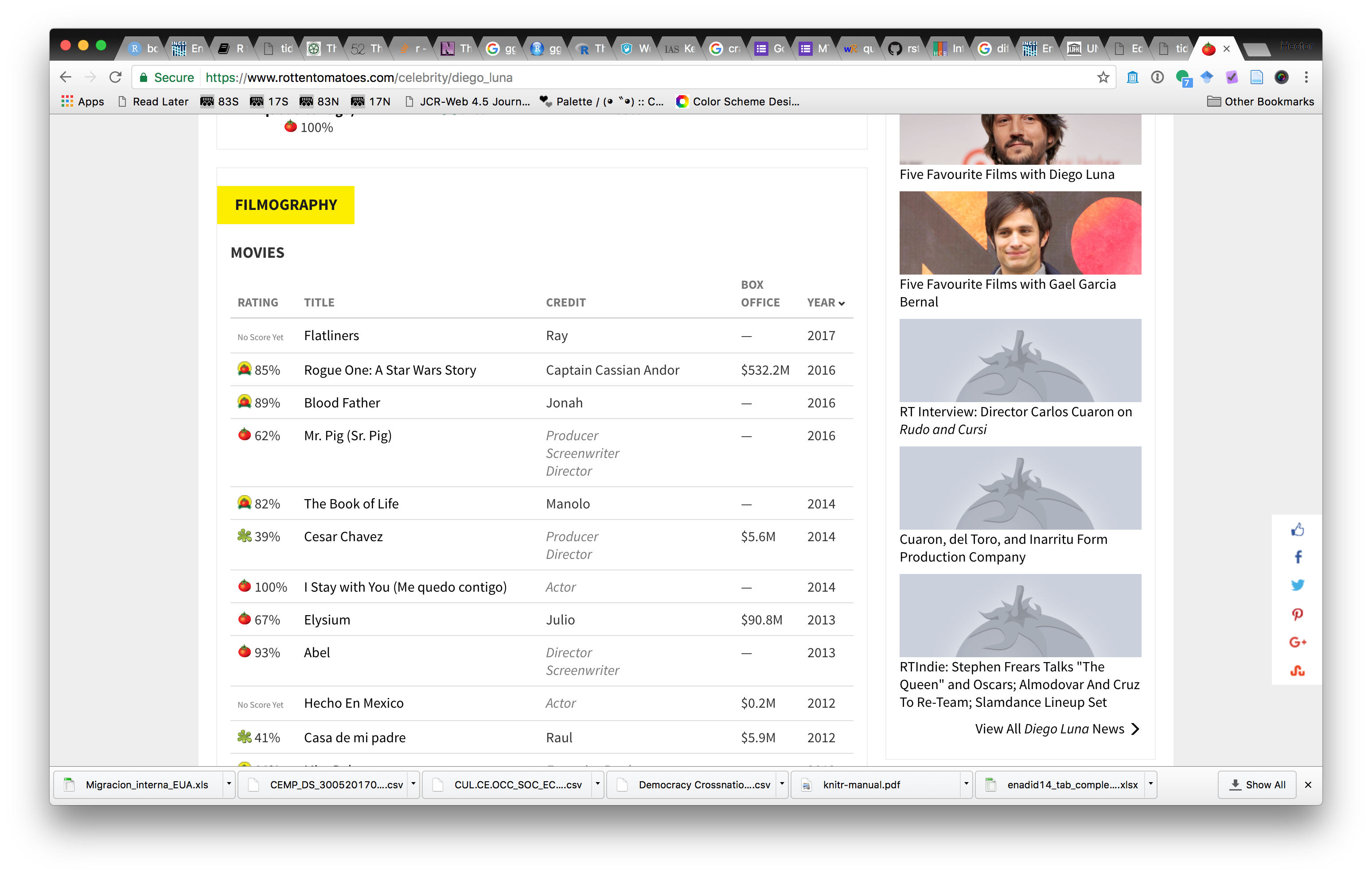
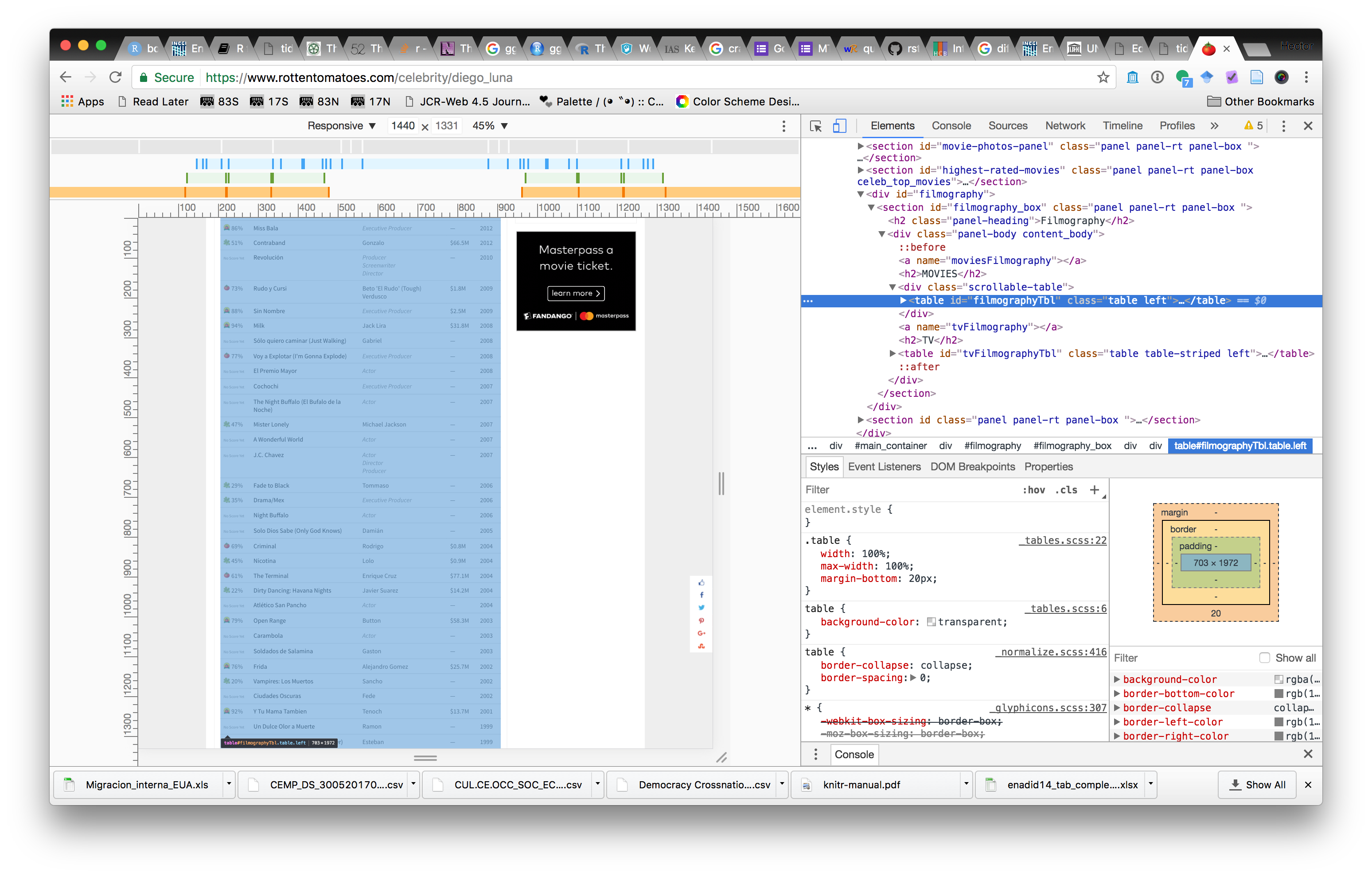
We can scrape ratings for his movies from this page. To do this we need to figure out how the HTML page’s markup can help us write R expressions to find this data in the page. Most web browsers have facilities to show page markup. In Google Chrome, you can use View>Developer>Developer Tools, and inspect the page markdown to find where the data is contained. In this example, we see that the data we want is in a <table> element in the page, with id filmographyTbl.
Now that we have that information, we can use the rvest package to scrape this data:
library(rvest)

url <- "https://www.rottentomatoes.com/celebrity/diego_luna"

dl_tab <- url %>%
  read_html() %>%
  html_node(".celebrity-filmography") %>%
  html_node("table") %>%
  html_table()

head(dl_tab)
## Rating Title
## 1 No Score Yet Wander Darkly
## 2 11% Berlin, I Love You
## 3 95% If Beale Street Could Talk
## 4 60% A Rainy Day in New York
## 5 No Score Yet Crow: The Legend
## 6 4% Flatliners
## Credit BoxOffice Year
## 1 Actor — 2020
## 2 Drag Queen — 2019
## 3 Pedrocito — 2019
## 4 Actor — 2019
## 5 Moth — 2018
## 6 Ray $16.9M 2017The main two functions we used here are html_node and html_table. html_node finds elements in the HTML page according to some selection criteria. Since we want the element with id=filmographyTbl we use the # selection operation since that corresponds to selection by id. Once the desired element in the page is selected, we can use the html_table function to parse the element’s text into a data frame.
The argument to the html_node function uses CSS selector syntax: https://www.w3.org/TR/CSS2/selector.html
On your own: If you wanted to extract the TV filmography from the page, how would you change this call?
16.2.1 Scraping from dirty HTML tables
We saw above how to extract data from HTML tables. But what if the data we want to extract is not cleanly formatted as a HTML table, or is spread over multiple html pages?
Let’s look at an example where we scrape titles and artists from billboard #1 songs: https://en.wikipedia.org/wiki/List_of_Billboard_Hot_100_number-one_singles_of_2017
Let’s start by reading the HTML markup and finding the document node that contains the table we want to scrape
library(rvest)
url <- "https://en.wikipedia.org/wiki/List_of_Billboard_Hot_100_number-one_singles_of_2017"
singles_tab_node <- read_html(url) %>%
  html_node(".plainrowheaders")
singles_tab_node
## {html_node}
## <table class="wikitable plainrowheaders" style="text-align: center">
## [1] <tbody>\n<tr>\n<th width="40">\n<abbr titl ...Since the rows of the table are not cleanly aligned, we need to extract each attribute separately. Let’s start with the dates in the first column. Since we noticed that the nodes containing dates have attribute scope we use the attribute CSS selector [scope].
## [1] "January 7\n"   "January 14\n"
## [3] "January 21\n"  "January 28\n"
## [5] "February 4\n"  "February 11\n"
Next, we extract song titles, first we grab the tr (table row) nodes and extract from each the first td node using the td:first-of-type CSS selector. Notice that this gets us the header row which we remove using the magrittr::extract function.
The title nodes also tell us how many rows this spans, which we grab from the rowspan attribute.
title_nodes <- singles_tab_node %>% html_nodes("tr") %>% html_node("td:first-of-type") %>% magrittr::extract(-1)
song_titles <- title_nodes %>% html_text()
title_spans <- title_nodes %>% html_attr("rowspan")
cbind(song_titles, title_spans) %>% head(10)
## song_titles title_spans
## [1,] "1059\n" NA
## [2,] "re\n" NA
## [3,] "1060\n" NA
## [4,] "1061\n" NA
## [5,] "re\n" "2"
## [6,] "[7]" NA
## [7,] "re\n" "11"
## [8,] "[9]" NA
## [9,] "[10]" NA
## [10,] "[11]" NATo get artist names we get the second data element (td) of each row using the td:nth-of-type(2) CSS selector (again removing the first entry in result coming from the header row)
artist_nodes <- singles_tab_node %>% html_nodes("tr") %>% html_node("td:nth-of-type(2)") %>% magrittr::extract(-1)
artists <-  artist_nodes %>% html_text()
artists %>% head(10)
## [1] "\"Starboy\"\n"
## [2] "\"Black Beatles\"\n"
## [3] "\"Bad and Boujee\"\n"
## [4] "\"Shape of You\" "
## [5] "\"Bad and Boujee\"\n"
## [6] NA
## [7] "\"Shape of You\" "
## [8] NA
## [9] NA
## [10] NANow that we’ve extracted each attribute separately we can combine them into a single data frame
billboard_df <- data_frame(month_day=dates, year="2017", song_title_raw=song_titles, title_span=title_spans,
                           artist_raw=artists)
## Warning: `data_frame()` is deprecated, use `tibble()`.
## This warning is displayed once per session.## # A tibble: 52 x 5
## month_day year song_title_raw title_span
## <chr> <chr> <chr> <chr>
## 1 "January… 2017 "1059\n" <NA>
## 2 "January… 2017 "re\n" <NA>
## 3 "January… 2017 "1060\n" <NA>
## 4 "January… 2017 "1061\n" <NA>
## 5 "Februar… 2017 "re\n" 2
## 6 "Februar… 2017 "[7]" <NA>
## 7 "Februar… 2017 "re\n" 11
## 8 "Februar… 2017 "[9]" <NA>
## 9 "March 4… 2017 "[10]" <NA>
## 10 "March 1… 2017 "[11]" <NA>
## # … with 42 more rows, and 1 more variable:
## # artist_raw <chr>This is by no means a clean data frame yet, but we will discuss how to clean up data like this in later lectures. We can now abstract these operations into a function that scrapes the same data for other years.
scrape_billboard <- function(year, baseurl="https://en.wikipedia.org/wiki/List_of_Billboard_Hot_100_number-one_singles_of_") {
  url <- paste0(baseurl, year)
  # find table node
  singles_tab_node <- read_html(url) %>%
    html_node(".plainrowheaders")

  # extract dates
  dates <- singles_tab_node %>% html_nodes("[scope]") %>% html_text()

  # extract titles and spans
  title_nodes <- singles_tab_node %>% html_nodes("tr") %>% html_node("td:first-of-type") %>% magrittr::extract(-1)
  song_titles <- title_nodes %>% html_text()
  title_spans <- title_nodes %>% html_attr("rowspan")

  # extract artists
  artist_nodes <- singles_tab_node %>% html_nodes("tr") %>% html_node("td:nth-of-type(2)") %>% magrittr::extract(-1)
  artists <-  artist_nodes %>% html_text()

  # make data frame
  data_frame(month_day=dates, year=year, song_title_raw=song_titles, title_span=title_spans,
                           artist_raw=artists)
}

scrape_billboard("2016")
## # A tibble: 53 x 5
## month_day year song_title_raw title_span
## <chr> <chr> <chr> <chr>
## 1 "January… 2016 "1048\n" 3
## 2 "January… 2016 "[4]" <NA>
## 3 "January… 2016 "[5]" <NA>
## 4 "January… 2016 "1049\n" 3
## 5 "January… 2016 "[7]" <NA>
## 6 "Februar… 2016 "[8]" <NA>
## 7 "Februar… 2016 "1050\n" <NA>
## 8 "Februar… 2016 "1051\n" <NA>
## 9 "Februar… 2016 "re\n" <NA>
## 10 "March 5… 2016 "1052\n" 9
## # … with 43 more rows, and 1 more variable:
## # artist_raw <chr>We can do this for a few years and create a (very dirty) dataset with songs for this current decade:
billboard_tab <- as.character(2010:2017) %>%
  purrr::map_df(scrape_billboard)

billboard_tab %>%
  head(20) %>%
knitr::kable("html")| month_day | year | song_title_raw | title_span | artist_raw |
|---|---|---|---|---|
| January 7 | 2012 | 1010 | 2 | “Sexy and I Know It” |
| January 14 | 2012 | [13] | NA | NA |
| January 21 | 2012 | re | 2 | “We Found Love” |
| January 28 | 2012 | [15] | NA | NA |
| February 4 | 2012 | 1011 | 2 | “Set Fire to the Rain” |
| February 11 | 2012 | [17] | NA | NA |
| February 18 | 2012 | 1012 | 2 | “Stronger (What Doesn’t Kill You)” |
| February 25 | 2012 | [19] | NA | NA |
| March 3 | 2012 | 1013 | NA | “Part of Me” |
| March 10 | 2012 | re | NA | “Stronger (What Doesn’t Kill You)” |
| March 17 | 2012 | 1014 | 6 | “We Are Young” |
| March 24 | 2012 | [22] | NA | NA |
| March 31 | 2012 | [23] | NA | NA |
| April 7 | 2012 | [24] | NA | NA |
| April 14 | 2012 | [25] | NA | NA |
| April 21 | 2012 | [7] | NA | NA |
| April 28 | 2012 | 1015 | 8 | “Somebody That I Used to Know” |
| May 5 | 2012 | [27] | NA | NA |
| May 12 | 2012 | [28] | NA | NA |
| May 19 | 2012 | [29] | NA | NA |
The function purrr::map_df is an example of a very powerful idiom in functional programming: mapping functions on elements of vectors. Here, we first create a vector of years (as strings) using as.character(2010:2017) we pass that to purrr::map_df which applies the function we create, scrape_billboard on each entry of the year vector. Each of these calls evaluates to a data_frame which are then bound (using bind_rows) to create a single long data frame. The tidyverse package purrr defines a lot of these functional programming idioms.
One more thing: here’s a very nice example of rvest at work: https://deanattali.com/blog/user2017/