27 Data Analysis with Geometry
A common situation in data analysis is that one has an outcome attribute (variable) \(Y\) and one or more independent covariate or predictor attributes \(X_1,\ldots,X_p\). One usually observes these variables for multiple “instances” (or entities).
(Note) As before, we use upper case to denote a random variable. To denote actual numbers we use lower case. One way to think about it: \(Y\) has not happened yet, and when it does, we see \(Y=y\).
One may be interested in various things:
- What effects do the covariates have on the outcome?
- How well can we describe these effects?
- Can we predict the outcome using the covariates?, etc…
27.1 Motivating Example: Credit Analysis
| default | student | balance | income |
|---|---|---|---|
| No | No | 729.5265 | 44361.625 |
| No | Yes | 817.1804 | 12106.135 |
| No | No | 1073.5492 | 31767.139 |
| No | No | 529.2506 | 35704.494 |
| No | No | 785.6559 | 38463.496 |
| No | Yes | 919.5885 | 7491.559 |
Task: predict account default What is the outcome \(Y\)? What are the predictors \(X_j\)?
We will sometimes call attributes \(Y\) and \(X\) the outcome/predictors, sometimes observed/covariates, and even input/output. We may call each entity an observation or example. We will denote predictors with \(X\) and outcomes with \(Y\) (quantitative) and \(G\) (qualitative). Notice \(G\) are not numbers, so we cannot add or multiply them. We will use \(G\) to denote the set of possible values. For gender it would be \(G=\{Male,Female\}\).
27.2 From data to feature vectors
The vast majority of ML algorithms we see in class treat instances as “feature vectors”. We can represent each instance as a vector in Euclidean space \(\langle x_1,\ldots,x_p,y \rangle\). This means:
- every measurement is represented as a continuous value
- in particular, categorical variables become numeric (e.g., one-hot encoding)
Here is the same credit data represented as a matrix of feature vectors
| default | student | balance | income |
|---|---|---|---|
| -1 | 1 | 1817.17118 | 24601.04 |
| 1 | 0 | 1975.65303 | 38221.84 |
| -1 | 1 | 296.46276 | 20138.25 |
| 1 | 1 | 1543.09958 | 18304.65 |
| 1 | 0 | 2085.58698 | 35657.23 |
| -1 | 0 | 59.96583 | 24889.25 |
27.3 Technical notation
Observed values will be denoted in lower case. So \(x_i\) means the \(i\)th observation of the random variable \(X\).
- Matrices are represented with bold face upper case. For example \(\mathbf{X}\) will represent all observed predictors.
- \(N\) (or \(n\)) will usually mean the number of observations, or length of \(Y\). \(i\) will be used to denote which observation and \(j\) to denote which covariate or predictor.
- Vectors will not be bold, for example \(x_i\) may mean all predictors for subject \(i\), unless it is the vector of a particular predictor \(\mathbf{x}_j\).
All vectors are assumed to be column vectors, so the \(i\)-th row of \(\mathbf{X}\) will be \(x_i'\), i.e., the transpose of \(x_i\).
27.4 Geometry and Distances
Now that we think of instances as vectors we can do some interesting operations.
Let’s try a first one: define a distance between two instances using Euclidean distance
\[d(x_1,x_2) = \sqrt{\sum_{j=1}^p(x_{1j}-x_{2j})^2}\]
27.4.1 K-nearest neighbor classification
Now that we have a distance between instances we can create a classifier. Suppose we want to predict the class for an instance \(x\).
K-nearest neighbors uses the closest points in predictor space predict \(Y\).
\[ \hat{Y} = \frac{1}{k} \sum_{x_k \in N_k(x)} y_k. \]
\(N_k(x)\) represents the \(k\)-nearest points to \(x\). How would you use \(\hat{Y}\) to make a prediction?

An important notion in ML and prediction is inductive bias. What assumptions we make about our data that allow us to make predictions. In KNN, our inductive bias is that points that are nearby will be of the same class. Parameter \(K\) is a hyper-parameter, it’s value may affect prediction accuracy significantly.
Question: which situation may lead to overfitting, high or low values of \(K\)? Why?
27.4.2 The importance of transformations
Feature scaling is an important issue in distance-based methods. In the example below, which of these two features will affect distance the most?
## Warning: `as_data_frame()` is deprecated, use `as_tibble()` (but mind the new semantics).
## This warning is displayed once per session.
27.5 Quick vector algebra review
A (real-valued) vector is just an array of real values, for instance \(x = \langle 1, 2.5, −6 \rangle\) is a three-dimensional vector.
Vector sums are computed pointwise, and are only defined when dimensions match, so
\[\langle 1, 2.5, −6 \rangle + \langle 2, −2.5, 3 \rangle = \langle 3, 0, −3 \rangle\].
In general, if \(c = a + b\) then \(cd = ad + bd\) for all vectors \(d\).
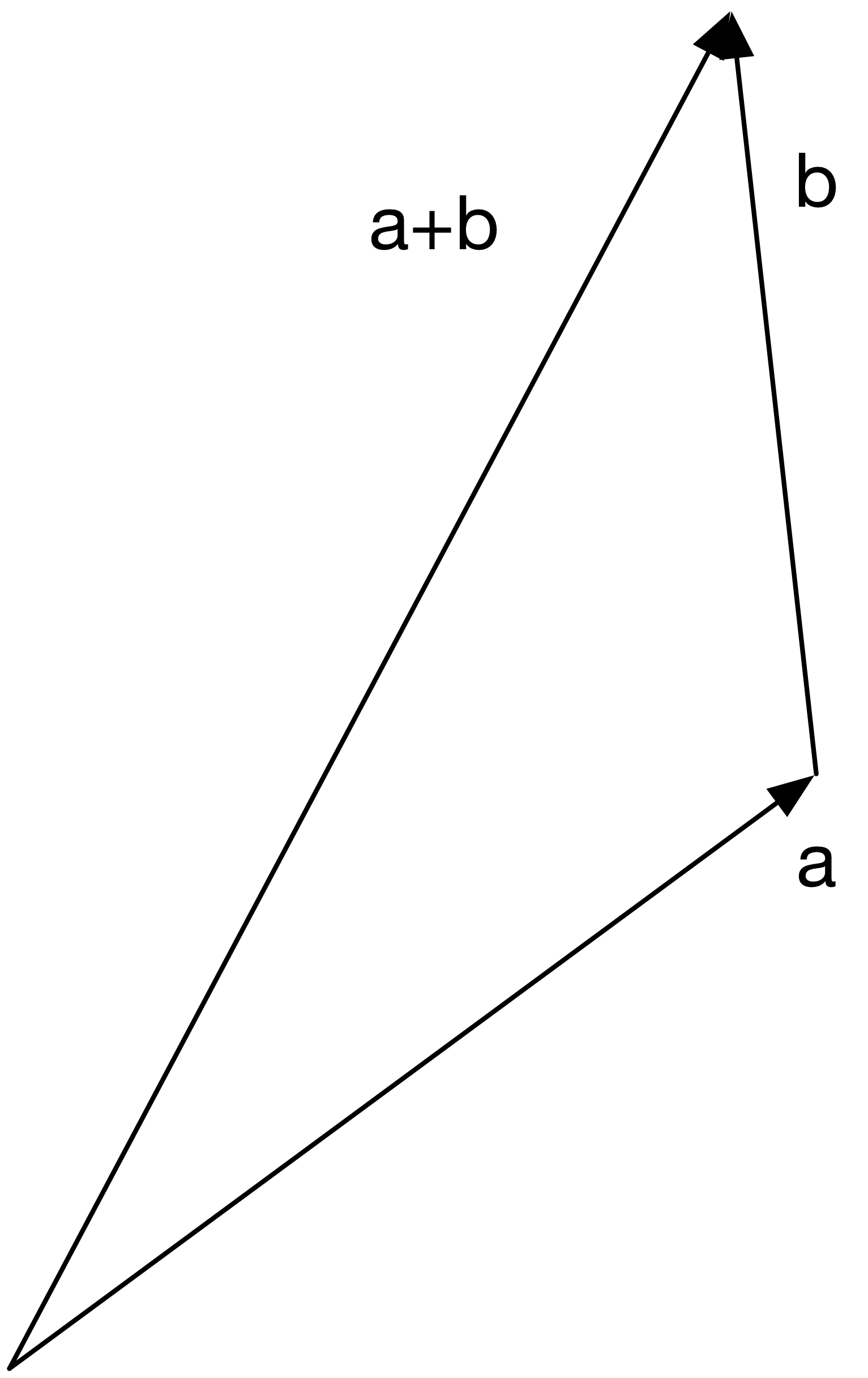
Vector addition can be viewed geometrically as taking a vector \(a\), then tacking on \(b\) to the end of it; the new end point is exactly \(c\).
Scalar Multiplication: vectors can be scaled by real values;
\[2\langle 1, 2.5, −6 \rangle = \langle 2, 5, −12\rangle\]
In general, \(ax = \langle ax_1, ax_2, \ldots, ax_p\rangle\)
The norm of a vector \(x\), written \(\|x\|\) is its length.
Unless otherwise specified, this is its Euclidean length, namely:
\[\|x\| = \sqrt{\sum_{j=1}^p x_j^2}\]
27.5.1 Quiz
Write Euclidean distance of vectors \(u\) and \(v\) as a vector norm
The dot product, or inner product of two vectors \(u\) and \(v\) is defined as
\[u'v = \sum_{j=1}^p u_i v_i\]
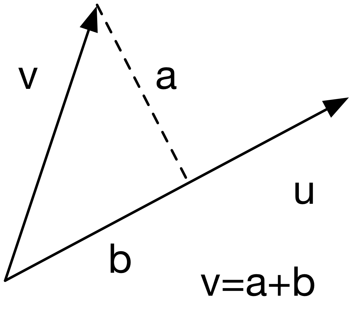
A useful geometric interpretation of the inner product \(v'u\) is that it gives the projection of \(v\) onto \(u\) (when \(\|u\|=1\)).
27.6 The curse of dimensionality
Distance-based methods like KNN can be problematic in high-dimensional problems
Consider the case where we have many covariates. We want to use \(k\)-nearest neighbor methods.
Basically, we need to define distance and look for small
multi-dimensional “balls”
around the target points. With many covariates this becomes
difficult.
Imagine we have equally spaced data and that each
covariate is in \([0,1]\). We want to something like kNN with a local focus
that uses
10% of the data in the local fitting.
If we have
\(p\) covariates and we are forming \(p\)-dimensional cubes, then each
side of the cube must have size \(l\) determined by \(l \times l \times \dots \times l = l^p = .10\).
If the number of covariates is p=10, then \(l = .1^{1/10} = .8\). So it
really isn’t local! If we reduce the percent of data we consider to
1%, \(l=0.63\). Still not very local.
If we keep reducing the size of the neighborhoods we will end up with very small number of data points in each average and thus predictions with very large variance.
This is known as the curse of dimensionality. Because of this so-called curse, it is not always possible to use KNN. But other methods, like Decision Trees, thrive on multidimensional data.
27.7 Summary
- We will represent many ML algorithms geometrically as vectors
- Vector math review
- K-nearest neighbors
- The curse of dimensionality