11 Tidy Data I: The ER Model
Some of this material is based on Amol Deshpande’s material: https://github.com/umddb/datascience-fall14/blob/master/lecture-notes/models.md
11.1 Overview
In this section we will discuss principles of preparing and organizing data in a way that is amenable for analysis, both in modeling and visualization. We think of a data model as a collection of concepts that describes how data is represented and accessed. Thinking abstractly of data structure, beyond a specific implementation, makes it easier to share data across programs and systems, and integrate data from different sources.
Once we have thought about structure, we can then think about semantics: what does data represent?
- Structure: We have assumed that data is organized in rectangular data structures (tables with rows and columns)
- Semantics: We have discussed the notion of values, attributes, and entities.
So far, we have used the following data semantics: a dataset is a collection of values, numeric or categorical, organized into entities (observations) and attributes (variables). Each attribute contains values of a specific measurement across entities, and entities collect all measurements across attributes.
In the database literature, we call this exercise of defining structure and semantics as data modeling. In this course we use the term data representational modeling, to distinguish from data statistical modeling. The context should be sufficient to distinguish the two uses of the term data modeling.
Data representational modeling is the process of representing/capturing structure in data based on defining:
- Data model: A collection of concepts that describes how data is represented and accessed
- Schema: A description of a specific collection of data, using a given data model
The purpose of defining abstract data representation models is that it allows us to know the structure of the data/information (to some extent) and thus be able to write general purpose code. Lack of a data model makes it difficult to share data across programs, organizations, systems that need to be able to integrate information from multiple sources. We can also design algorithms and code that can significantly increase efficiency if we can assume general data structure. For instance, we can preprocess data to make access efficient (e.g., building a B-Tree on a field).
A data model typically consists of:
- Modeling Constructs: A collection of concepts used to represent the structure in the data. Typically we need to represent types of entities, their attributes, types of relationships between entities, and relationship attributes
- Integrity Constraints: Constraints to ensure data integrity (i.e., avoid errors)
- Manipulation Languages: Constructs for manipulating the data
We desire that models are sufficiently expressive so they can capture real-world data well, easy to use, and lend themselves to defining computational methods that have good performance.
Some examples of data models are
- Relational, Entity-relationship model, XML…
- Object-oriented, Object-relational, RDF…
- Current favorites in the industry: JSON, Protocol Buffers, Avro, Thrift, Property Graph
Why have so many models been defined? There is an inherent tension between descriptive power and ease of use/efficiency. More powerful, expressive, models can be applied to represent more datasets but also tend to be harder to use and query efficiently.
Typically there are multiple levels of modeling. Physical modeling concerns itself with how the data is physically stored. Logical or Conceptual modeling concerns itself with type of information stored, the different entities, their attributes, and the relationships among those. There may be several layers of logical/conceptual models to restrict the information flow (for security and/or ease-of-use):
- Data independence: The idea that you can change the representation of data w/o changing programs that operate on it.
- Physical data independence: I can change the layout of data on disk and my programs won’t change
- index the data
- partition/distribute/replicate the data
- compress the data
- sort the data
11.2 The Entity-Relationship and Relational Models
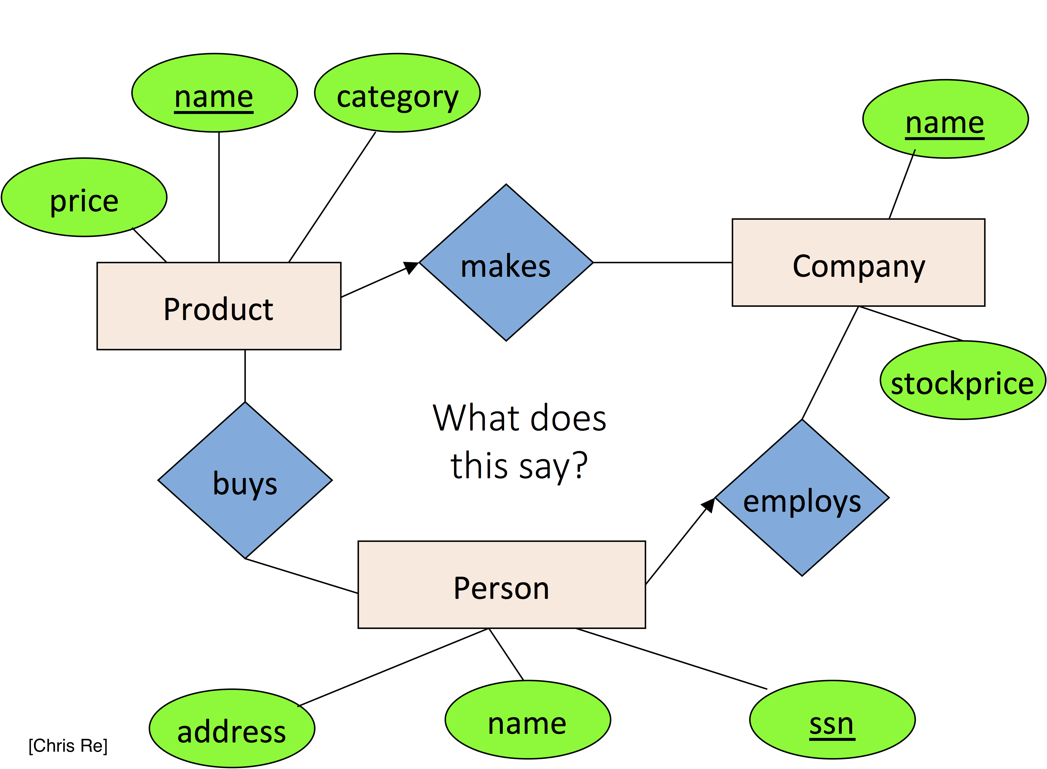
The fundamental objects in this formalism are entities and their attributes, as we have seen before, and relationships and relationship attributes. Entities are objects represented in a dataset: people, places, things, etc. Relationships model just that, relationships between entities.
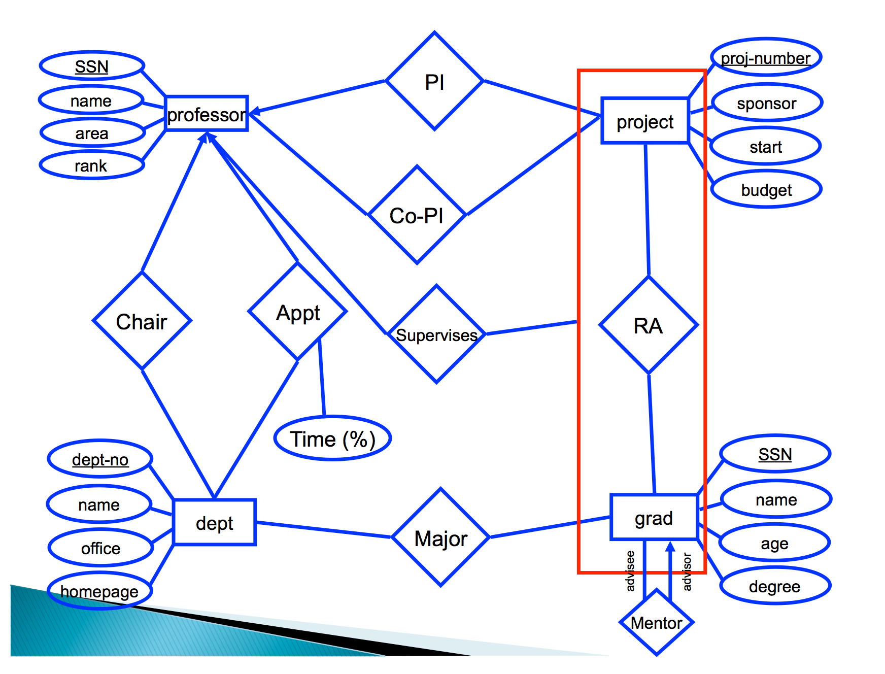
Here, rectangles are entitites, diamonds and edges indicate relationships. Circles describe either entity or relationship attributes. Arrows are used indicate multiplicity of relationships (one-to-one, many-to-one, one-to-many, many-to-many):
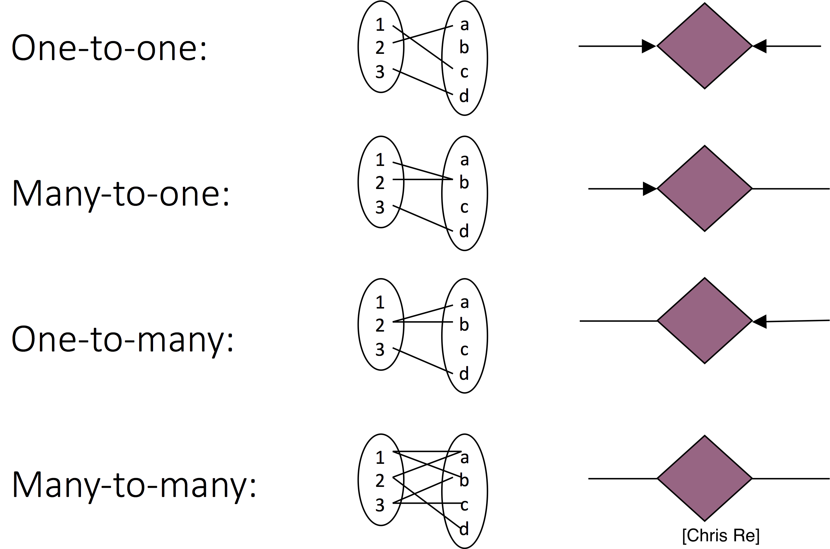
Relationships are defined over pairs of entities. As such, relationship \(R\) over sets of entities \(E_1\) and \(E_2\) is defined over the cartesian product \(E_1 \times E_2\). For example, if \(e_1 \in E_1\) and \(e_2 \in E_2\), then \((e_1, e_2) \in R\).
Arrows specify how entities participate in relationships. In particular, an arrow pointing from an entity set \(E_1\) (square) into a relationship over \(E_1\) and \(E_2\) (diamond) specifies that entities in \(E_1\) appear in only one relationship pair. That is, there is a single entity \(e_2 \in E_2\) such that \((e_1,e_2) \in R\).
Think about what relationships are shown in this diagram?
In databases and general datasets we work on, both Entities and Relationships are represented as Relations (tables) such that a unique entity/relationship is represented by a single tuple (the list of attribute values that represent an entity or relationship).
This leads to the natural question of how are unique entities determined or defined. Here is where the concept of a key comes in. This is an essential aspect of the Entity-Relationship and Relational models.
11.2.1 Formal introduction to keys
- Attribute set \(K\) is a superkey of relation \(R\) if values for \(K\) are sufficient to identify a unique tuple of each possible relation \(r(R)\)
- Example:
{ID}and{ID,name}are both superkeys of instructor
- Example:
- Superkey \(K\) is a candidate key if \(K\) is minimal
- Example:
{ID}is a candidate key for Instructor
- Example:
- One of the candidate keys is selected to be the primary key
- Typically one that is small and immutable (doesn’t change often)
- Primary key typically highlighted
- Foreign key: Primary key of a relation that appears in another relation
{ID}from student appears in takes, advisor- student called referenced relation
- takes is the referencing relation
- Typically shown by an arrow from referencing to referenced
- Foreign key constraint: the tuple corresponding to that primary key must exist
- Imagine:
- Tuple:
('student101', 'CMSC302')in takes - But no tuple corresponding to ‘student101’ in student
- Tuple:
- Also called referential integrity constraint
- Imagine:
11.2.1.1 Keys: Examples
- Married(person1-ssn, person2-ssn, date-married, date-divorced)
- Account(cust-ssn, account-number, cust-name, balance, cust-address)
- RA(student-id, project-id, superviser-id, appt-time, appt-start-date, appt-end-date)
- Person(Name, DOB, Born, Education, Religion, …)
- Information typically found on Wikipedia Pages
- President(name, start-date, end-date, vice-president, preceded-by, succeeded-by)
- Info listed on Wikipedia page summary
- Rider(Name, Born, Team-name, Coach, Sponsor, Year)
- Tour de France: Historical Rider Participation Information
11.3 Tidy Data
Later in the course we will use the term Tidy Data to refer to datasets that are represented in a form that is amenable for manipulation and statistical modeling. It is very closely related to the concept of normal forms in the ER model and the process of normalization in the database literature.
Here we assume we are working in the ER data model represented as relations: rectangular data structures where
- Each attribute (or variable) forms a column
- Each entity (or observation) forms a row
- Each type of entity (observational unit) forms a table
Here is an example of a tidy dataset:
## # A tibble: 6 x 19
##    year month   day dep_time sched_dep_time
##   <int> <int> <int>    <int>          <int>
## 1  2013     1     1      517            515
## 2  2013     1     1      533            529
## 3  2013     1     1      542            540
## 4  2013     1     1      544            545
## 5  2013     1     1      554            600
## 6  2013     1     1      554            558
## # … with 14 more variables: dep_delay <dbl>,
## #   arr_time <int>, sched_arr_time <int>,
## #   arr_delay <dbl>, carrier <chr>,
## #   flight <int>, tailnum <chr>, origin <chr>,
## #   dest <chr>, air_time <dbl>, distance <dbl>,
## #   hour <dbl>, minute <dbl>, time_hour <dttm>
it has one entity per row, a single attribute per column. Notice only information about flights are included here (e.g., no airport or airline information other than the name) in these observations.