26 Multivariate probability
26.1 Joint and conditional probability
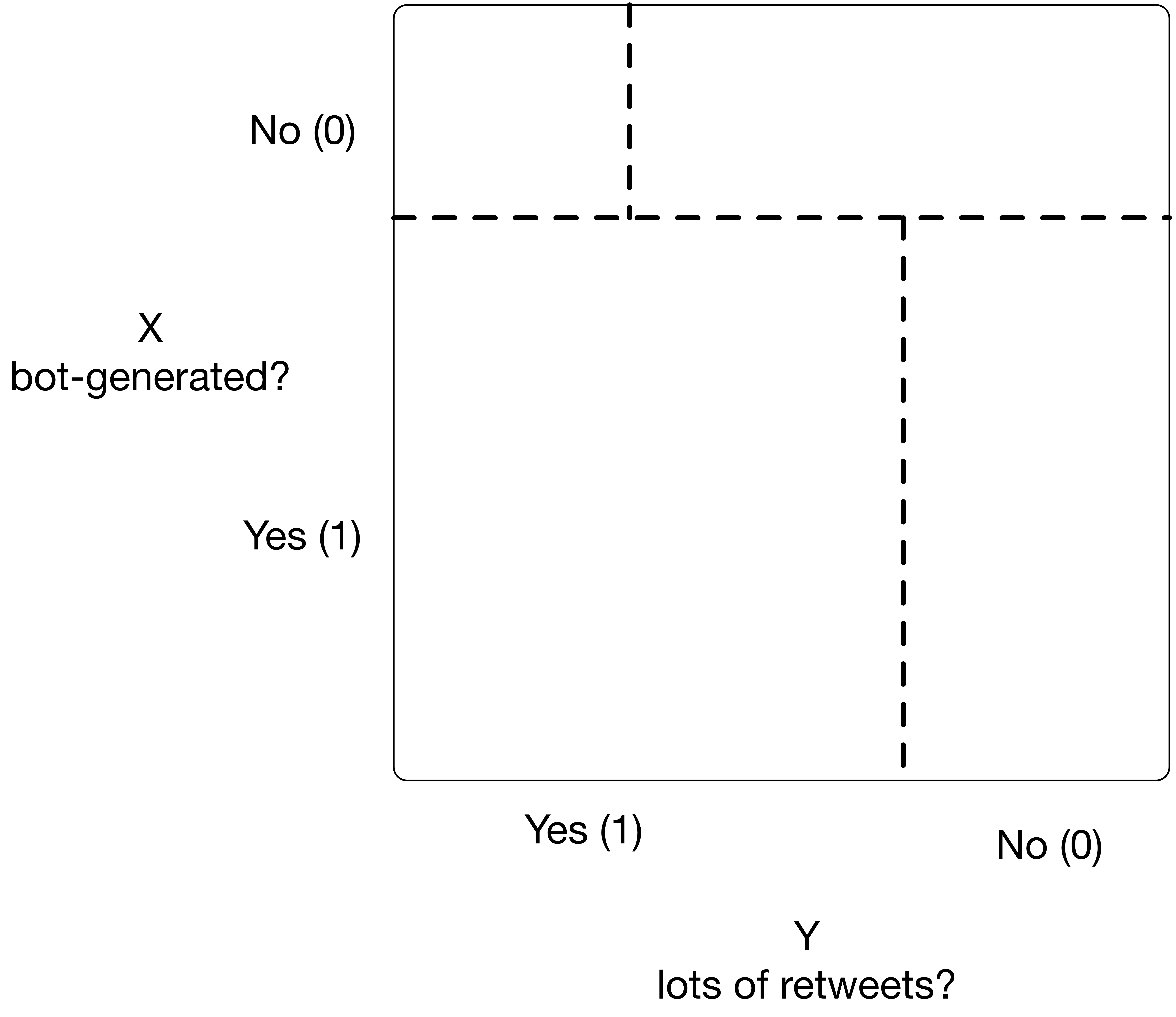
Suppose that for each tweet I sample I can also say if it has a lot of retweets or not. So, I have another binary random variable \(Y \in \{0,1\}\) where \(Y=1\) indicates the sampled tweet has a lot of retweets. (Note, we could say \(Y\sim \mathrm{Bernoulli}(p_Y))\). So we could illustrate the population of “all” tweets as
We can talk of the joint probability distribution of \(X\) and \(Y\): \(p(X=x, Y=y)\), where random variables \(X\) and \(Y\) can take values from domains \(\mathcal{D}_X\) and \(\mathcal{D}_Y\) respectively. Here we have the same conditions as we had for univariate distributions:
- \(p(X=x,Y=y)\geq 0\) for all combination of values \(x\) and \(y\), and
- \(\sum_{(x,y) \in \mathcal{D}_X \times \mathcal{D}_Y} p(X=x,Y=y) = 1\)
We can also talk about conditional probability where we look at the probability of a tweet being bot-generated or not, conditioned on wether it has lots of retweets or not:
\[ p(X=x | Y=y) \]
which also needs to satisfy the properties of a probability distribution. So to make sure
\[ \sum_{x \in \mathcal{D}_X} p(X=x|Y=y) = 1 \]
we define
\[ p(X=x | Y=y) = \frac{p(X=x,Y=y)}{p(Y=y)} \]
Here we use the important concept of marginalization, which follows from the properties of joint probability distribution we saw above: \(\sum_{x \in \mathcal{D}_X} p(X=x, Y=y) = p(Y=y)\).
This also lets us talk about independence: if the probabilty of a tweet being bot-generated does not depend on a tweet having lots of retweets, that is \(p(X=x) = p(X=x|Y=y)\) for all \(y\), then we say \(X\) is independent of \(Y\).
Consider the tweet diagram above, is \(X\) independent of \(Y\)? What would the diagram look like if \(X\) was independent of \(Y\)?
One more note, you can also see that for independent variables, the joint probability has an easy form \(p(X=x,Y=y)=p(X=x)p(Y=y)\), which generalizes to more than two independent random variables.
26.2 Bayes’ Rule
One extremely useful and important rule of probability follows from our definitions of conditional and joint probability above. Bayes’ rule is pervasive in Statistics, Machine Learning and Artificial Intelligence. It is a very powerful tool to talk about uncertainty, beliefs, evidence, and many other technical and philosophical matters. It is however, of extreme simplicity.
All Bayes’ Rule states is that
\[ p(X=x|Y=y) = \frac{p(Y=y|X=x)p(X=x)}{p(Y=y)} \] which follow directly from our definitions above. One very common usage of Bayes’ Rule is that it let’s us define one conditional probability distribution based on another probability distribution. This is useful is the latter is easier to reason about, or estimate. For example, it may be hard to reason about \(p(X=x|Y=y)\) in our tweet example. If you know a tweet has a lot retweets \((Y=1)\), what can you say about the probability that it is bot-generated, i.e., \(p(X=1|Y=1)\)? Maybe not much, tweets have lots of retweets for many reasons. However, it may be easier to reason about the reverse: if I tell you a tweet is bot-generated \((X=1)\), what can you say about the probability that it has a lot of retweets, i.e., \(p(Y=1|X=1)\). That may be easier to reason about, at least bot-generated tweets are designed to get lots of retweets. At minimum, it’s easier to estimate because we can get a training set of bot-generated tweets and estimate this conditional probability.
Bayes’ Rule tells us how to get the hard to reason about (or estimate) conditional probability \(p(X=x|Y=y)\) in terms of the conditional probability that is easier to reason about (or estimate) \(p(Y=y|X=x)\). This is the basis of the Naive Bayes prediction method, which we’ll revisit briefly later on.
26.3 Conditional expectation
With conditional probabilty we can start talking about conditional expectation, which generalizes the concept of expectation we saw before. For example, the conditional expected value (conditional mean) of \(X\) given \(Y=y\) is
\[ \mathbb{E} [ X|Y=y ] = \sum_{x \in \mathcal{D}_X} x p(X=x|Y=y) \]
This notion of conditional expectation, which follows from conditional probability, will serve as the basis for our Machine Learning method studies in the next few lectures!
26.4 Maximum likelihood
One last note. We saw before how we estimated a parameter from matching expectation from a probability model with what we observed in data. The most popular method of estimation uses a similar idea: given data \(x_1,x_2,\ldots,x_n\) and an assumed model of their distribution, e.g., \(X_i\sim \mathrm{Bernoulli}(p)\) for all \(i\), and they are iid, let’s find the value of parameter \(p\) that maximizes the likelihood (or probability) of the data we observe under this assumed probability model.
We call the resulting estimate the maximum likelihood estimate. Here are some fun exercises to try:
- Given a sample \(x_1\) with \(X_1 \sim N(\mu,1)\), show that the maximum likelihood estimate of \(\mu\), \(\hat{\mu}=x_1\).
It is most often convinient to minimize negative log-likelihood instead of maximizing likelihood. So in this case:
\[ \begin{align} -\mathscr{L}(\mu) & = - \log p(X_1=x_1) \\ {} & = \log{\sqrt{2\pi}} + \frac{1}{2}(x_1 - \mu)^2 \end{align} \]
To minimize this function of \(\mu\) we can ignore all terms that are independent of \(\mu\), and concentrate only on minimizing the last term. Now, this term is always positive, so the smallest value it can have is 0. So, we minimize it by setting \(\hat{\mu}=x_1\).
- Given a sample \(x_1,x_2,\ldots,x_n\) of \(n\) iid random variables with \(X_i \sim N(\mu,1)\) for all \(i\), show that the maximum likelihood estimate of \(\mu\), \(\hat{\mu}=\overline{x}\) the sample mean!
Here we would follow a similar approach, write out the negative log likelihood as a function \(f(\mu;x_i)\) of \(\mu\) that depends on data \(x_i\). Two useful properties here are:
- \(p(X_1=x_1,X_2=x_2,\ldots,X_n=x_n)=p(X_1=x_1)p(X_2=x_2)\cdots p(X_n=x_n)\), and
- \(\log \prod_i f(\mu;x_i) = \sum_i \log f(\mu;x_i)\)
Then find a value of \(\mu\) that minimizes this function. Hint: we saw this when we showed that the sample mean is the minimizer of total squared distance in our exploratory analysis unit!